install.packages("usethis")
usethis::use_course("https://github.com/benjaminhlina/shortest_path_example/archive/refs/heads/master.zip")0.1 Our Objectives
The purpose of this vignette is to create the shortest distance among acoustic telemetry receivers within a confined boundary such as a lake, river, delta, or oceanscape. This workflow can be adapted to find the distance between any two points within a confined boundary.
You can download and unzip this vignette using the following code:
0.2 Disclaimer
This vignette uses {gdistance}, {raster}, and {sp} which as of October 2023 were retired. Please use the vignette using {pathroutr} for the timing being until I can update this vignette with using {terra}.
0.3 Load shapefile and receiver locations
We will first load all the packages we need, we will use {gdistance} to find the shortest paths, {sf} to find the distances of those shortest paths.
# ---- load packages ----
{
  library(dplyr)
  library(gdistance)
  library(ggplot2)
  library(here)
  library(purrr)
  library(raster)
  library(readr)
  library(sf)
  library(sp)
  library(tibble)
  library(tidyr)
  make_line <- function(lon, lat, llon, llat) {
    st_linestring(matrix(c(lon, llon, lat, llat), 2, 2))
  }
}
We will bring bring in our shapefile. This vignette will use Big Sissabagama Lake as it is the lake I grew up fishing on in Wisconsin, USA. Please replace with the shapefile of your desired body of water.
lake <- st_read(dsn = here("Data",
                           "shapefile",
                           "."),
                layer = "sissabagama_lake")
Important that you convert to the correct UTM zone. For the vignette we are using UTM zone 15 N. Adjust your UTM zone accordingly.
lake_utm <- st_transform(lake, crs = 32615)Create SpatialPloygonDataFrame we will use it to create a raster that will be a transition layer for paths to move across. We will use lake_utm as we need our raster layer in UTMs.
lake_spd <- as_Spatial(lake_utm)We will then bring in our receiver locations. Replace rl_sum_sf with your receiver locations as a RDS or csv file type or whatever you use to document receiver locations.
rl_sum_sf <- read_rds(here("Data",
                           "receiver locations",
                           "rl_sum_sf.rds"))
Convert to UTMs for plotting purposes and make sure you use the correct UTM zone.
rl_sum_utm <- st_transform(rl_sum_sf, crs = 32615)0.4 Rasterize shapefile
We will look at lake SpatialPointsDataFrame via plot, then determine the boundary box (bbox) and save it as an object named ext.
plot(lake_spd)

# determine the extent of the SpatialPointsDataFrame
ext <- extent(lake_spd)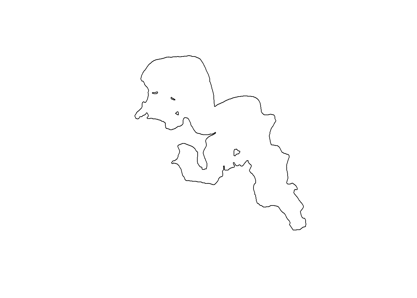
Then we will create the raster, it is important here to control the res argument as that will result in varied resolution. For the vignette I used a resolution of 5 which represents 5 m since we are using UTMs. Using a more fine-scale resolution such as 5 m can be computationally intensive so for large systems scale this value up.
s <- raster(lake_spd, res = 5)
# remove and change NA values to fit within the extent
s <- rasterize(x = lake_spd, y = s, field = 1)

# plot raster to make sure it looks appropriate
plot(s)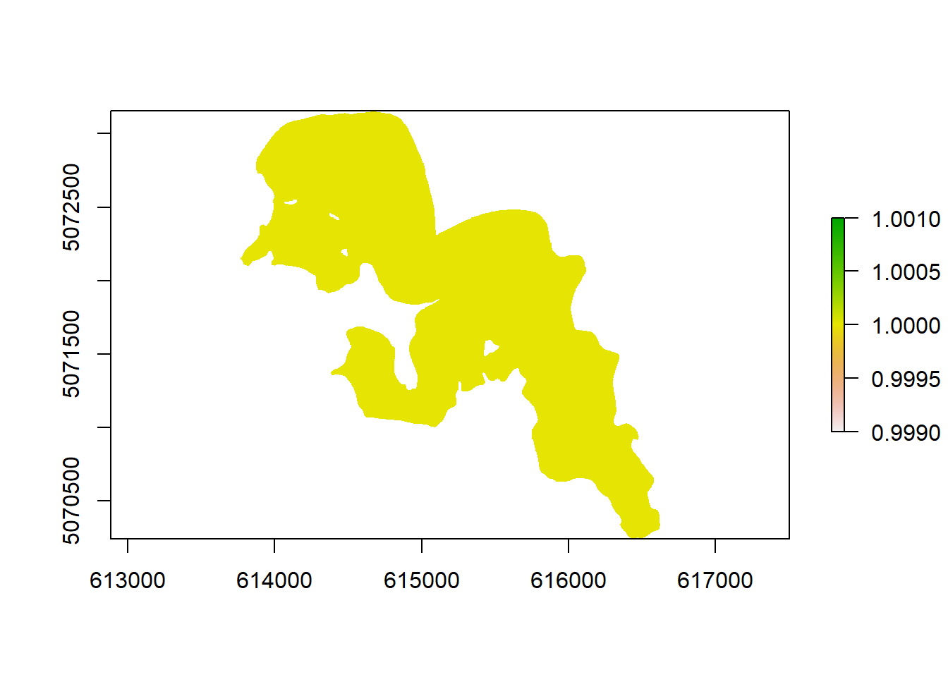
The last step is to create the transition layer. Directions will be queens move of 16 spaces. If in a larger systems direction could be reduced from queens space to rook or king, 4 or 8 to reduce computational complexity and speed.
trans <- transition(x = s, transitionFunction = mean, directions = 16)0.5 Create every combination of paths for every receiver
First we will convert receiver location which is a sf object to a tibble with each location combination.
prep_path <- rl_sum_sf %>%
  mutate(
    lon = st_coordinates(.)[,"X"],# grab lon
    lat = st_coordinates(.)[,"Y"],# grab lat
  ) %>%
  st_drop_geometry() %>% # drop sf
  # once geometry removed create to and from lat longs
  mutate(llon = lon,
         llat = lat,
         lonlat = paste0(lon, ",", lat),
         llonllat = paste0(llon, ",", llat)) %>%
  dplyr::select(-lon, -lat, -llon, -llat) %>%
  expand(lonlat, llonllat) %>% # expand for each to and from combo
  separate(lonlat, c("lon", "lat"), ",") %>%
  separate(llonllat, c("llon", "llat"), ",")
prep_path has all of the path combinations but we lose the names of the receivers and which paths go from one receiver to another. We are going to add that information back in by creating an object called rec_order
rec_order <- prep_path %>%
  left_join(
    rl_sum_sf %>%
      mutate(
        lon = st_coordinates(.)[,"X"], # grab lon
        lat = st_coordinates(.)[,"Y"]  # grab lat
      ) %>%
      st_drop_geometry() %>% # remove sf
      rename(from = rec_name) %>%  # Line up from names
      dplyr::select(from, lon, lat) %>%
      mutate(across(.cols = c(lon, lat), as.character)) , by = c("lon", "lat"),
    multiple = "all"
  ) %>%
  left_join(
    rl_sum_sf %>%
      mutate(
        lon = st_coordinates(.)[,"X"]
      ) %>%
      st_drop_geometry() %>%
      rename(to = rec_name,
             llon = lon) %>% # join for the tos
      dplyr::select(to, llon) %>%
      mutate(llon = as.character(llon)), by = c("llon"),
    multiple = "all"
  ) %>%
  mutate(
    from_to = paste0(from, "-", to),
    id = 1:nrow(.)
  ) %>%
  dplyr::select(id, from, to, from_to, lon, lat, llon, llat) %>%
  mutate(across(.col = c(lon, lat, llon, llat), as.numeric))
Awesome! We have all of our combinations with their names and we now know which paths go from one receiver to another. The only issue is all of points are in decimal degrees with a CRS of WGS 84, we need to convert this into to UTMs.
Be sure to choose the correct UTM zone here. This vignette uses UTM zone 15 north but for other uses you will have to change the UTM zone.
rec_order_utm <- st_as_sf(rec_order,
                          coords = c("lon", "lat"),
                          crs = st_crs(rl_sum_sf)) %>%
  st_transform(crs = 32615) %>%
  mutate(
    lon = st_coordinates(.)[,"X"], # grab lon
    lat = st_coordinates(.)[,"Y"]  # grab lat
  ) %>%
  st_drop_geometry() %>%
  st_as_sf(., coords = c("llon", "llat"),
           crs = st_crs(rl_sum_sf)) %>%
  st_transform(crs = 32615) %>%
  mutate(
    llon = st_coordinates(.)[,"X"], # grab lon
    llat = st_coordinates(.)[,"Y"]  # grab lat
  ) %>%
  st_drop_geometry()
0.6 Make shortest paths
We will first split our combinations into individual end points, then use purrr::map() to iterate over each combination and use the shortestPath() function to calculate the shortest path for every combination.
We then will transform the output of this which are SpatialLinesDataFrame to sf objects. Important note here is to change the CRS to your specific CRS UTM zone.
rec_dist_sf <- rec_order_utm %>%
  split(.$id) %>%
  map(possibly(~ shortestPath(trans,
                              c(.$llon, .$llat),
                              c(.$lon, .$lat),
                              output = "SpatialLines"), NA)) %>%
  map(possibly(~ st_as_sf(., crs = 32615), NA)) %>% # u will need to replace CRS
  bind_rows(.id = "id") %>%
  mutate(
    cost_dist = as.numeric(st_length(.))
  )
0.7 Add in metadata of paths start and end desitantions
First we will change the id column to a character to be able to line up the data properly.
rec_order_names <- rec_order_utm %>%
  mutate(
    id = as.character(id)
  )
Next we will use left_join() from {dplyr} to connect each path’s metadata.
rec_dist_sf <- rec_dist_sf %>%
  left_join(rec_order_names, by = "id") %>%
  dplyr::select(id, from:llon, cost_dist, geometry)
0.8 Plot
We will use ggplot to look at our paths. Lets first check if paths go to the right locations and then we will plot the whole thing.
ggplot() +
  geom_sf(data = lake_utm) +
  geom_sf(data = rec_dist_sf %>%
            filter(from_to %in% "3-12")
          , aes(colour = cost_dist), size = 1) +
  geom_sf_label(data = rl_sum_utm , size = 4, aes(label = rec_name)) +
  scale_colour_viridis_c(name = "Cost Distance (m)", option = "B") +
  theme_void()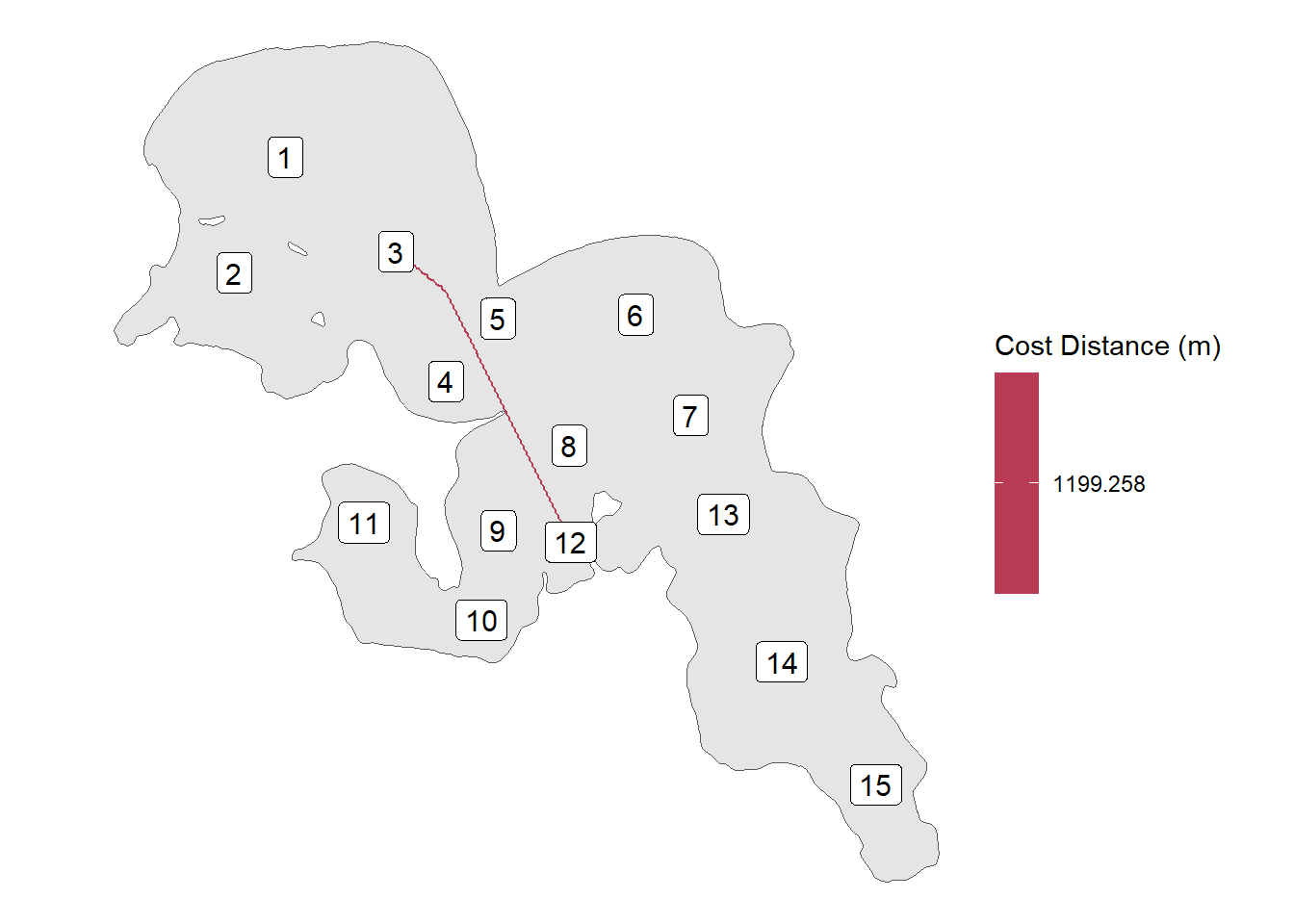
ggplot() +
geom_sf(data = lake_utm) +
geom_sf(data = rec_dist_sf, aes(colour = cost_dist), size = 1) +
geom_sf(data = rl_sum_utm , size = 4) +
scale_colour_viridis_c(name = "Cost Distance (m)", option = "B") +
theme_void()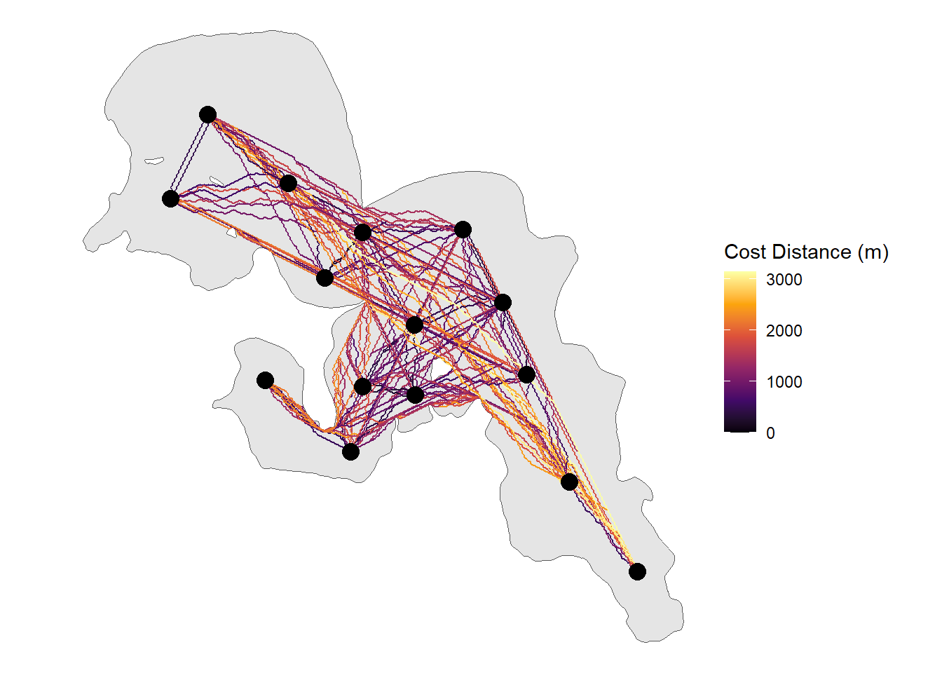 From here the
 sf object can be kept together or ripped apart to determine the distance or path a fish could swim within the system along with a whole host of other potential implications (e.g. interpolated paths).
Credit: R. Lennox, PhD, Incoming Science Director - OTN for the original ideas around this script.