install.packages("devtools")
devtools::install_github("dill/soapcheckr")0.1 Our Objectives
The purpose of this vignette is to demonstrate an effective workflow while using {soapcheckr} to efficiently make a soap-film smoother for a Generalized Additive Model (GAM) using the package {mgcv}. Soap-film smoothers are really useful when trying to model a variable within a 3-dimensional space (e.g., bathymetry of a lake; Gavin Simpson Blog Post). They can be used for all sorts of data but are quite complex and difficult to setup. {soapcheckr} tries to make this process a little easier. This vignette will walk through several different examples using example data sets loaded when loading {soapcheckr} and {mgcv}. We strongly encourage going through both examples, as the first provides a general background on soap-films within a simple boundary and the second a more complex example within a more complex boundary.
0.2 Example 1: Making a soap-film smoother for a Simple boundary - Ramsay’s horseshoe
If we were wanting to make a soap-film smoother for a boundary that does not have any inner boundaries (e.g., a lake without an island) we can use {soapcheckr} to assess our single boundary and the potential knots we want to smooth over.
0.2.1 Install {soapcheckr}
0.2.2 Load packages
We will use some data manipulation functions from {dplyr} and some spatial functions from {sf} to first check if we can make a soap-film using {soapcheckr} and second to run a GAM using {mgcv} with a soap-film smoother.
{
  library(broom.mixed)
  library(fitdistrplus)
  library(dplyr)
  library(ggplot2)
  library(gratia)
  library(mgcv)
  library(purrr)
  library(soapcheckr)
  library(sf)
}
0.2.3 Check if we can make a soap-film for Ramsey’s horseshoe
We will load Ramsey’s horseshoe from {mgcv} and make it a list within a list to sufficiently create the boundary a soap-film smoother needs within a GAM.
fsb <- list(fs.boundary())We can then can check the boundary using soap_check().
soap_check(fsb)
#> [1] TRUEWe can see that soap_check() returns TRUE indicating that we can use this boundary to make a soap-film smoother. soap_check() will assess if the boundary supplied, has any overlapping polygons and is in the correct structure for a soap-film smoother to be run in {mgcv}.
0.2.4 Check if the data and the evenly spaced knots fall within the boundary
Sometimes knots are too close to the boundary, resulting with errors from the model that look like this:
Error in crunch.knots(ret$G, knots, x0, y0, dx, dy) :
knot 1 is on or outside boundary
It can be tedious and annoying to try to figure out which knots and/or data points are causing issues. The below workflow will demonstrate how to effectively remove knots and/or data points that result in the above error within the GAM.
We will use expand.grid() to create an equally spaced grid of knots. Then we remove knots outside of the boundary using inSide() from {mgcv}. There still may be knots that are too close to the boundary that will cause for a soap-film smoother to not work.
# create knots
knots <- expand.grid(x = seq(min(fsb[[1]]$x),
                             max(fsb[[1]]$x), len = 15),
                     y = seq(min(fsb[[1]]$y) + 0.05,
                             max(fsb[[1]]$y), len = 10))
x <- knots$x
y <- knots$y

# identify the knots that are outside the boundary
ind <- inSide(fsb, x = x, y = y)
# remove knots outside the boundary
knots <- knots[ind, ]
We will also create some fake data to test the model. We will use a uniform distribution to make our test data and a response variable will be created using fs.test(). We will use inSide() to remove data that fall outside our boundary.
set.seed(0)
n <- 600

# Our x and y data
x <- runif(n) * 5 - 1
y <- runif(n) * 2 - 1

# create our response variable
z <- fs.test(x, y, b = 1)

## remove outsiders

ind <- inSide(fsb, x = x, y = y)

z <- z + rnorm(n) * 0.3 ## add noise

# create the data we want to model
dat <- data.frame(z = z[ind],
                  x = x[ind],
                  y = y[ind])
However, there still may be knots and/or data points that are too close to the boundary. One can go through, one-by-one and remove the offending knots as crunch.knots() finds them, but that’s a bit tedious. Enter soap_check() and autocruncher(), with the former allowing one to visually check what knots and/or data will causes issues and the latter identifying the index location of the offending knots or data points. If the knot dataframe has column names other than x and y, we need to supply soapcheckr() those names using the arguments x_name and y_name, respectfully.
soap_check(fsb, knots = knots)
#> Warning in soap_check(fsb, knots = knots): Knots 1, 13, 66, 93 are outside the
#> boundary.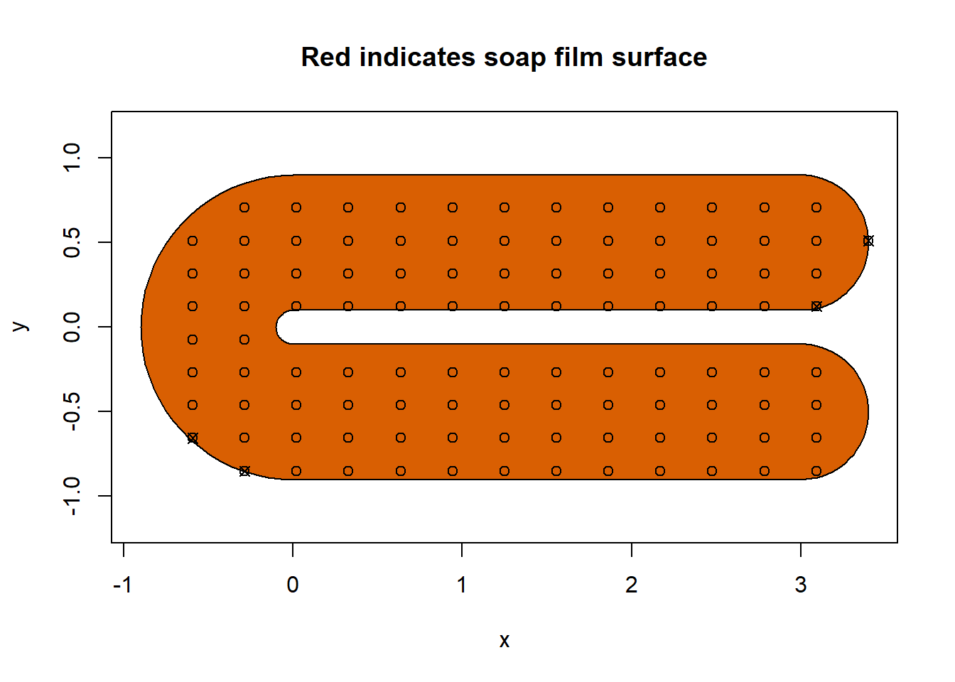
#> [1] TRUEWe can see that there four offending knots that we can subsequently remove using autocruncher(). This function will return the indices of the knots that would cause issues. If the knot dataframe has column names other than x and y, we need supply those column names to the arguments xname and yname, respectfully. Note that you need to set the k and nmax arguments in autocruncher() to be the same as your planned value in gam().
crunch_index <- autocruncher(fsb, knots, k = 30)
crunch_index
#> [1]  1 13 66 93

# remove knots that are problematic
knots <- knots[-crunch_index, ]
We can use soap_check() again to check if knots all fall within the boundary.
soap_check(fsb, knots = knots)
#> [1] TRUEAnd they do! Congratulations!
0.2.5 Check the data
We can also use soap_check() to check if our data falls within the boundary, but soap_check() only cares about the coordinates you want to supply the soap-film. So first we will create a secondary dataframe that has the response variable, z, removed from it.
dat_2 <- dat[, 2:3]
soap_check(fsb, data = dat_2)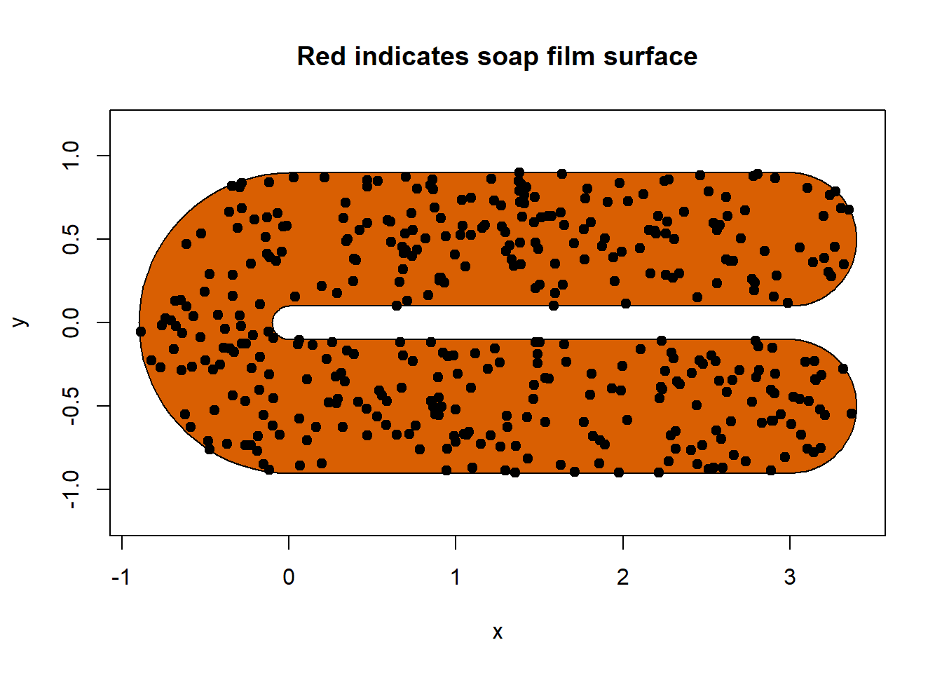
#> [1] TRUECongrats we can see our data doesn’t fall too closely to boundary and is within the boundary.
0.2.6 Run the model
Between data, knots, and boundary all column names must be the same for the model to work. Prior to running confirm that they are all the same.
m <- gam(z ~ s(x, y, k = 30 , bs = "so",
               xt = list(bnd = fsb)),
         knots = knots,
         data = dat)
Next, check main effects of the model.
anova(m)Then visually check the model effects using draw() from {gratia}
draw(m)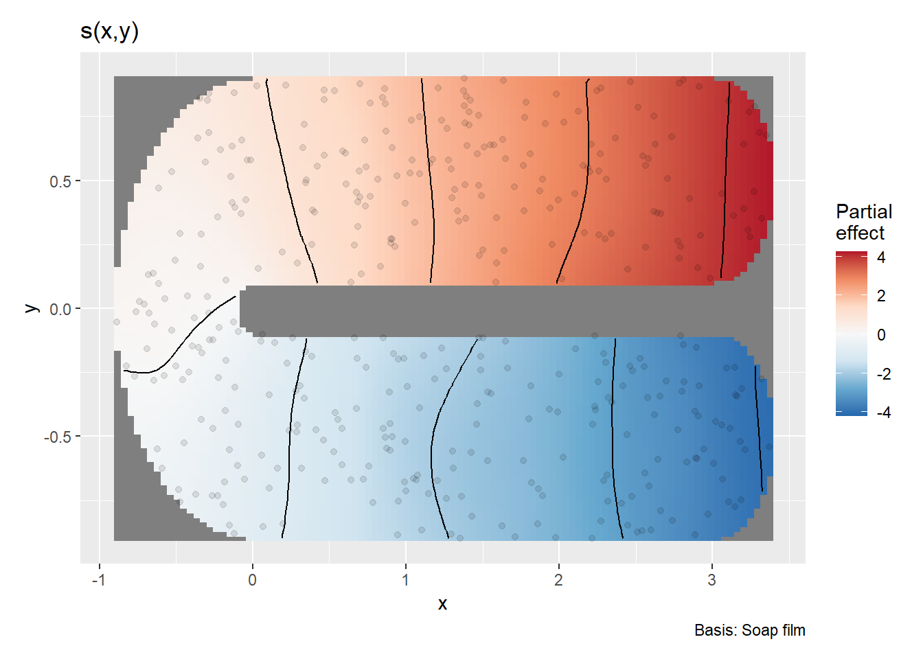
Lastly, check the model fit using appraise() from {gratia}
appraise(m)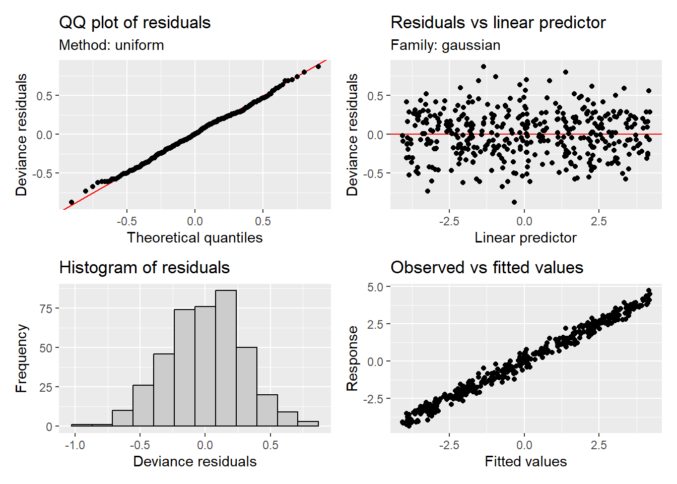
We can see the model fits well and is appropriate for the example data. Now that you’ve walked through a simple boundary, we will go to a more complex boundary example. More than likely you will be working with a complex boundary. The below walk through can be applied to a simple boundary as well.
0.3 Example 2: Making a soap-film smoother for a more complex boundary.
More than likely you will have your boundary as a sf object. To convert that sf object into the boundary list needed by {mgcv} and {soapcheckr}, we will have to do some conversions. First that boundary might not be in the correct coordinate reference system (CRS). To create a soap-film smoother we need to use a CRS that for one unit change in either dimension (i.e., x and y) are equal. For example using latitude and longitude in decimal degrees with a WGS 84 projection will not work because one unit of change in either direction is not equal. Therefore, we will need to use a CRS that is based on equal units. The most common CRS to do this is UTMs, if the boundary is already in UTMs great, if not see below.
0.3.1 Convert CRS
The more complex boundary that we will load through {soapcheckr} is a lake from northern Wisconsin, Sissabagama Lake. I grew up fishing on this lake which is where initially became interested and passionate about aquatic ecosystems, fish, and fisheries management. This lake falls within UTM zone 15N that can also be refereed to as ESPG: 32615, but your boundary will more than likely fall into a different CRS. You can look up ESPG codes here.
sissabagama_lake_sf <- sissabagama_lake_sf %>%
  st_transform(crs = 32615)
0.3.2 Convert to boundary list
We need to create the list of lists of the boundaries from the sf object that we will supply to the soap-film smoother.
Our example lake has a geometry column that is a POLYGON. We need to be able to split that into each polygon (i.e., islands) that we will create the boundary list from. We can do this by first casting our geometry into MULTIPOINT and assigning each MULTIPOINT row an ID value.
bnd_pt_sf <- sissabagama_lake_sf %>%
  dplyr::select(geometry) %>%
  st_cast("MULTIPOINT") %>%
  mutate(
    id = 1:nrow(.)
  )
Next we will split our sf object and iterate over each MULTIPOINT geometry to first cast to individual POINT geometry and extract each x and y coordinates. It is important in this step that the names of the coordinates are x and y.
bnd_pt <- bnd_pt_sf %>%
  split(.$id) %>%
  purrr::map(~ st_cast(.x, "POINT") %>%
               mutate(
                 x = st_coordinates(.)[,"X"],
                 y = st_coordinates(.)[,"Y"]
               ) %>%
               st_drop_geometry() %>%
               dplyr::select(-id)
  )
We now have a list of dataframes split by each polygon’s x and y coordinates that have had the id column removed. We then need to create a vector that is id number of each polygon. In this case it’s 1-5, we can use length() of our list of dataframes to easily create the end of our numerical vector.
We will then iterate over our list and bind them all together to get our lists and lists of our polygon boundaries.
nr <- 1:length(bnd_pt)

sissabagama_bnd_ls <- lapply(nr, function(n) as.list.data.frame(bnd_pt[[n]]))
0.3.3 Check if the boundary list works
We will check the boundary list using soap_check()
soap_check(sissabagama_bnd_ls)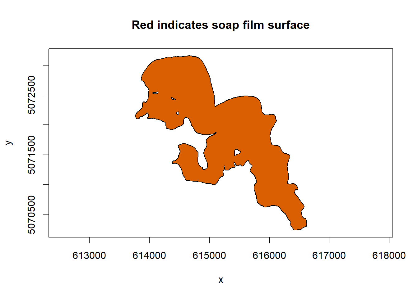
#> [1] TRUEsoap_check returns back TRUE so our more complex boundary will work for our soap-film smoother. One thing that I’ve always loved about this lake is how it looks like person!
0.3.4 Make knots for a more complex boundary using {sf}
We can use st_make_grid() to create a grid of equally spaced points across the boundary box of our example sf object of Sissabagama Lake. Remember a soap-film smoother needs equally spaced knots to smooth over. Our sf object is in UTMs which is great becasue then each grid point in this case is 200 m away from each other. Depending on the size of the boundary and system you can change 200 to whatever value makes sense (e.g., large system, further spaced knots, small system, closer spaced knots/this is suggestion but do whatever makes sense).
lake_grid <- sissabagama_lake_sf %>%
  st_make_grid(cellsize = 200, square = TRUE, what = "centers") %>%
  st_as_sf()

st_geometry(lake_grid) <- "geometry"
We will then remove all the knots that fall outside the boundary by using st_intersection().
lake_intesects <- st_intersection(sissabagama_lake_sf, lake_grid)Next we will create our knot dataframe by extracting the lon and lat of each point and then dropping the geometry column and selecting our lon and lat columns.
lake_knots <- lake_intesects %>%
  mutate(
    lon = st_coordinates(.)[,"X"],
    lat = st_coordinates(.)[,"Y"]
  ) %>%
  st_drop_geometry() %>%
  as.data.frame() %>%
  dplyr::select(lon, lat)
Now that we have our knots we can check to see if there are any knots that fall too close to the boundary using soap_check().
soap_check(sissabagama_bnd_ls, knots = lake_knots,
           x_name = "lon", y_name = "lat")
#> Warning in soap_check(sissabagama_bnd_ls, knots = lake_knots, x_name = "lon", :
#> Knots 42, 63, 68 are outside the boundary.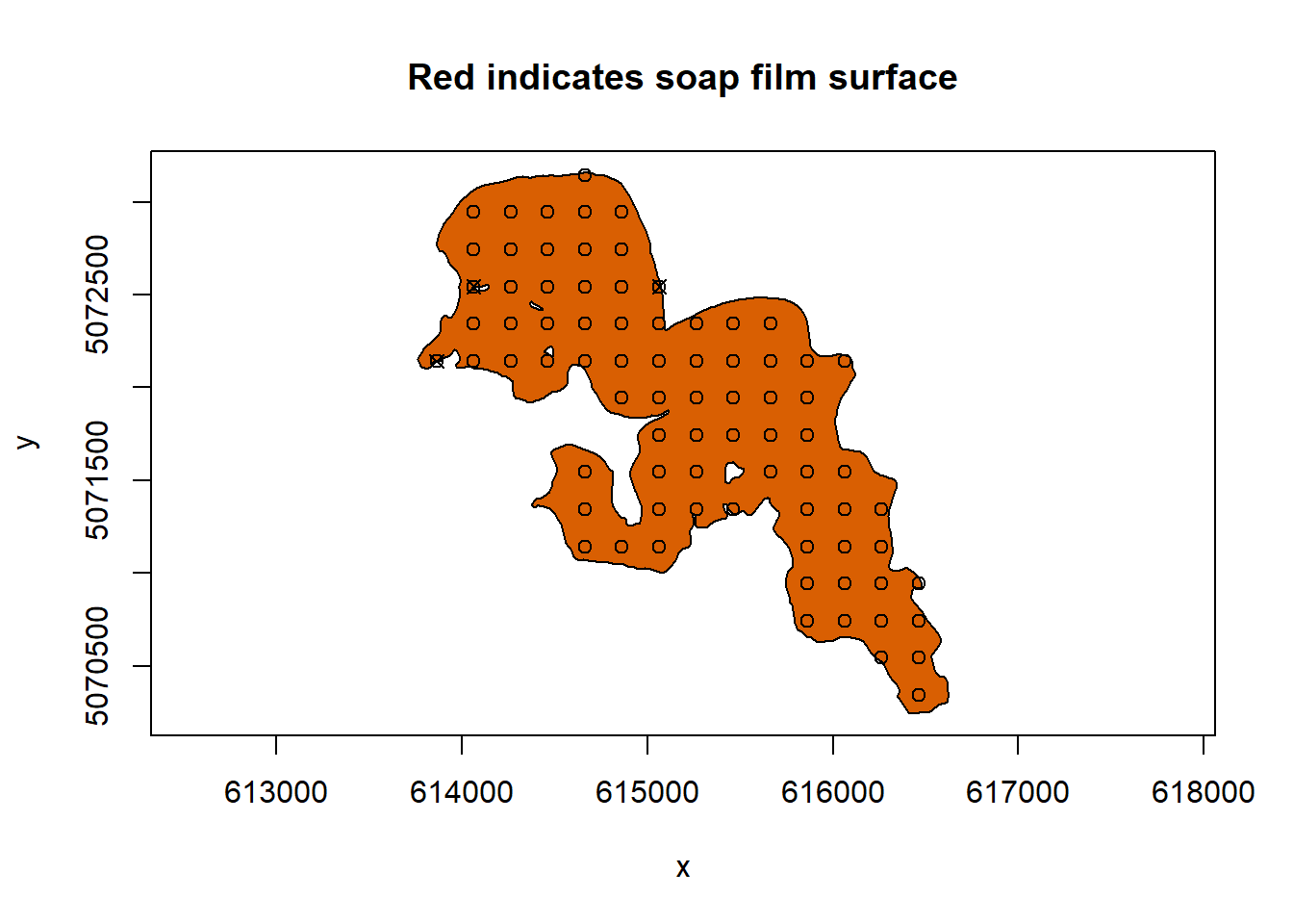
#> [1] TRUEWe can see that there are a few knots that are too close to the boundary. We can remove them using autocruncher()
crunch_ind <- autocruncher(sissabagama_bnd_ls, lake_knots,
                           xname = "lon", yname = "lat")
crunch_ind
#> [1] 42 63 68

# remove knots that are problematic
lake_knots <- lake_knots[-crunch_ind, ]
Now that those knots have been removed we can recheck our knots using soap_check().
soap_check(sissabagama_bnd_ls, knots = lake_knots,
           x_name = "lon", y_name = "lat")
#> [1] TRUECongratulations! We have knots and a boundary that we can supply our model.
0.3.5 Sissabagama example dataset
We will bring our sampled depths at given locations for Sissabagama lake. This data was generated by referencing the contour map supplied by the Wisconsin DNR. We will first remove depth to check if the data points all fall within our boundary using soap_check().
sissabagama_bath_pt <- sissabagama_bath %>%
  dplyr::select(-depth)

soap_check(sissabagama_bnd_ls, data = sissabagama_bath_pt)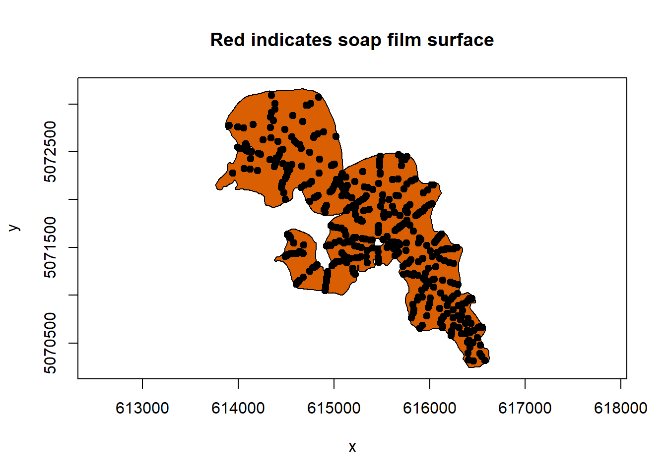
#> [1] TRUEThen we will assess the distribution of the data to determine which distribution the model should use to fit the data to. We will use functions from {fitdistrplus}.
depths <- sissabagama_bath$depth
descdist(depths)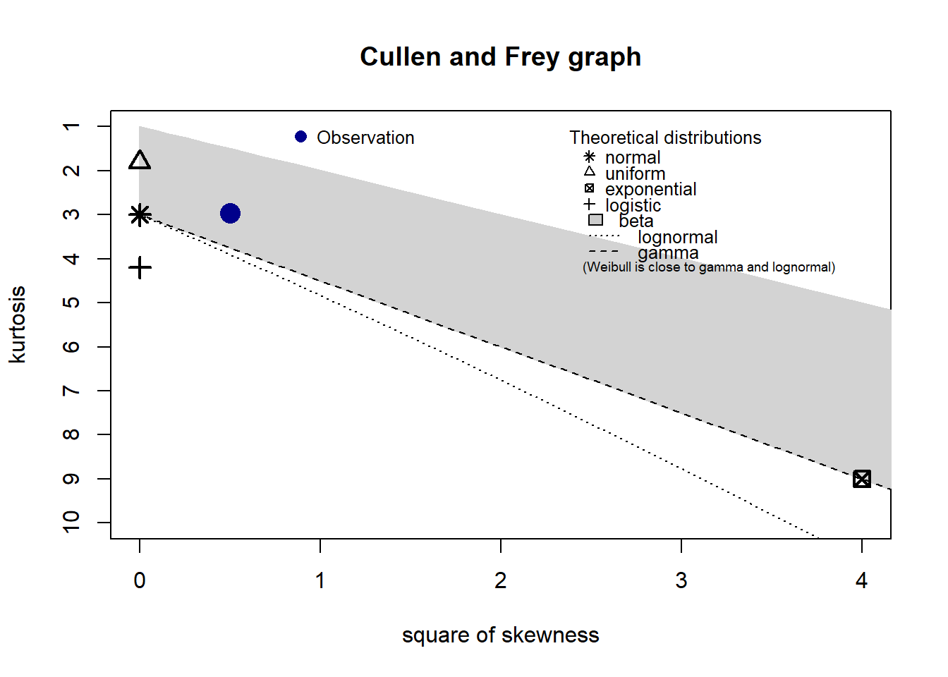
#> summary statistics
#> ------
#> min:  3   max:  48
#> median:  15
#> mean:  15.29438
#> estimated sd:  9.983594
#> estimated skewness:  0.7078068
#> estimated kurtosis:  2.964066
Skewness and kurtosis of our example data indicates that a model using a Gamma error distribution will likely fit.
fit_gamma <- fitdist(depths, distr = "gamma", method = "mme")
plot(fit_gamma)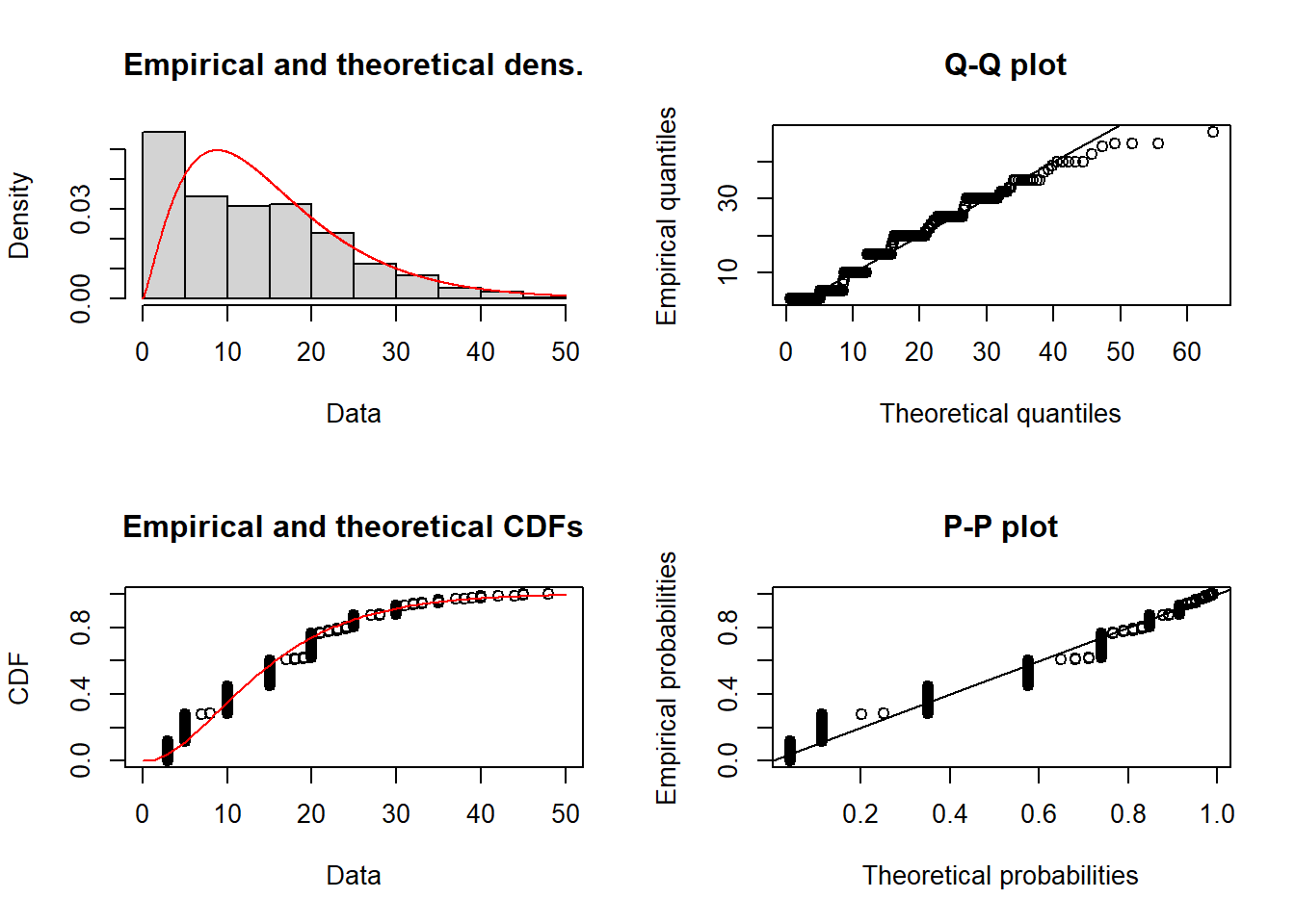
We can see the depth data will likely fit a Gamma error distribution and therefore our GAM will use a Gamma error distribution.
0.3.6 Run the model
Prior to running our GAM with a soap-film smoother we need to add one last thing to our boundary list. We need to add the variable f to every boundary polygon within our boundary list. This variable indicates to the soap-film smoother that our response variable is 0 right at the boundary, otherwise the soap-film smoother does not know what to do when it hits the boundary.
names(lake_knots) <- c("x", "y")

sissabagama_bnd_ls <- lapply(nr,
                             function(n)
                               sissabagama_bnd_ls[[n]] <- c(
                                 sissabagama_bnd_ls[[n]],
                                 list(f = rep(0, length(sissabagama_bnd_ls[[n]]$x))
                                 )
                               )
)
We can now successfully run our GAM with a soap-film smoother.
m1 <- gam(depth ~ s(x, y,
                    bs = "so",
                    xt = list(bnd = sissabagama_bnd_ls)),
          family = Gamma(link = "identity"),
          knots = lake_knots,
          data = sissabagama_bath)
We can evaluate the main of the model using anova()
anova(m1)
#>
#> Family: Gamma
#> Link function: identity
#>
#> Formula:
#> depth ~ s(x, y, bs = "so", xt = list(bnd = sissabagama_bnd_ls))
#>
#> Approximate significance of smooth terms:
#>          edf Ref.df     F p-value
#> s(x,y) 57.47  76.00 16.51  <2e-16
Next we can evaluate partial effects of the model using summary()
summary(m1)
#>
#> Family: Gamma
#> Link function: identity
#>
#> Formula:
#> depth ~ s(x, y, bs = "so", xt = list(bnd = sissabagama_bnd_ls))
#>
#> Parametric coefficients:
#>             Estimate Std. Error t value Pr(>|t|)
#> (Intercept)   2.8408     0.2074    13.7   <2e-16 ***
#> ---
#> Signif. codes:  0 '***' 0.001 '**' 0.01 '*' 0.05 '.' 0.1 ' ' 1
#>
#> Approximate significance of smooth terms:
#>          edf Ref.df     F p-value
#> s(x,y) 57.47     76 16.51  <2e-16 ***
#> ---
#> Signif. codes:  0 '***' 0.001 '**' 0.01 '*' 0.05 '.' 0.1 ' ' 1
#>
#> R-sq.(adj) =  0.786   Deviance explained = 76.8%
#> GCV = 0.15835  Scale est. = 0.12696   n = 445
We can evaluate the partial effects of the model using draw() from {gratia}
draw(m1)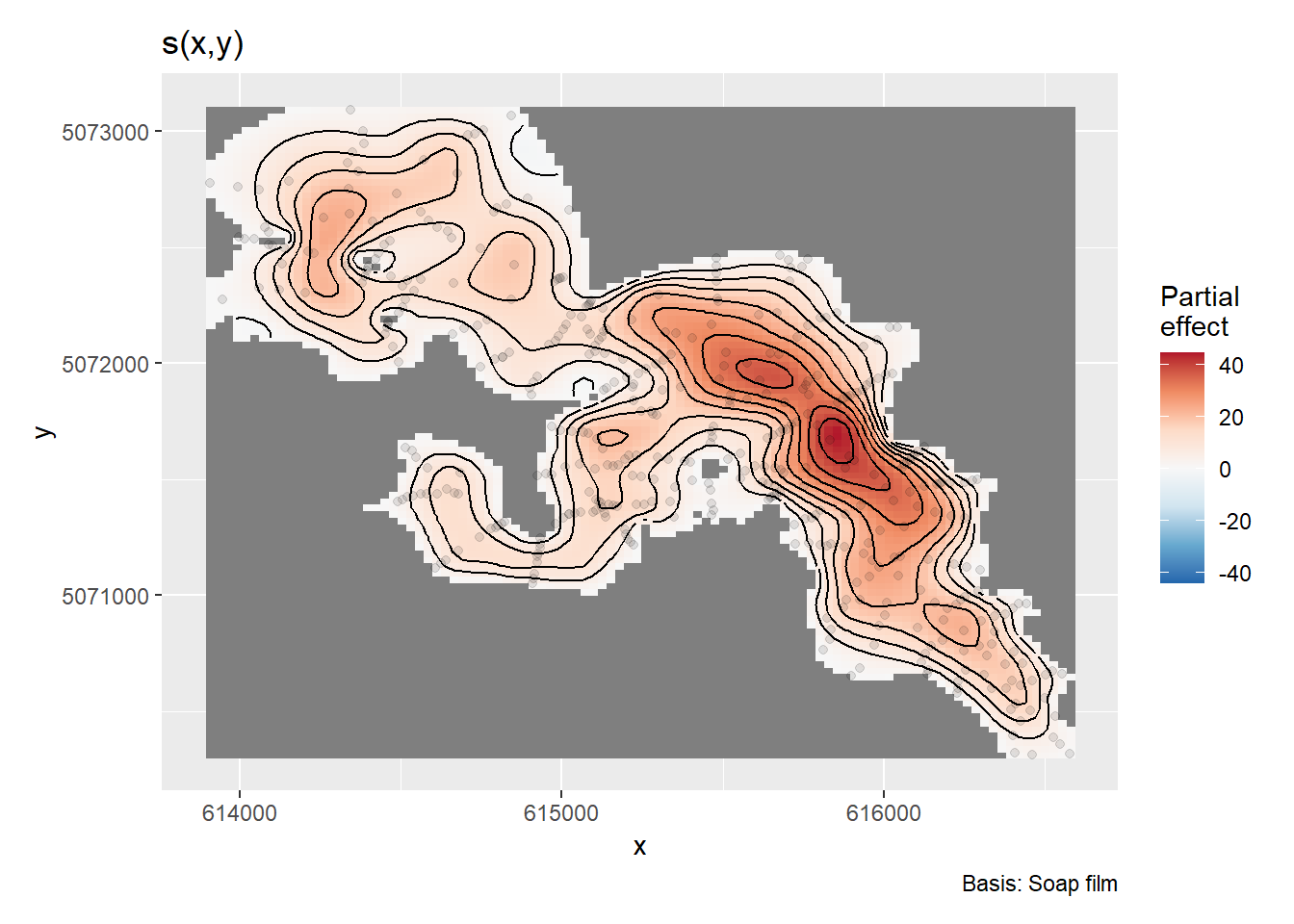
We can evaluate how well the model fit is to the data using appraise() also from {gratia}
appraise(m1)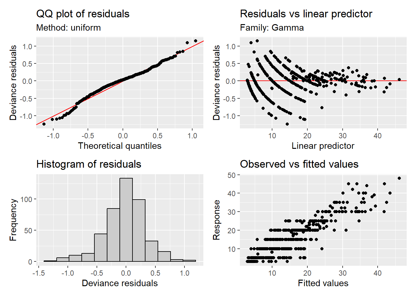
0.3.7 Plot our predicted results
We will first create a 10 m grid from our sf object of our boundary. Depending on the size of the boundary you can change the grid size distance to whatever distance makes sense (i.e., if the system is large you may want to increase the cellsize).
lake_pred <- sissabagama_lake_sf %>%
  st_make_grid(cellsize = 10, square = TRUE, what = "centers") %>%
  st_as_sf()
st_geometry(lake_pred) <- "geometry"
After creating the grid that we will predict values from we will need to remove any points that fall outside our polygon boundary.
lake_pred <- st_intersection(lake_pred, sissabagama_lake_sf) %>%
  dplyr::select(geometry)
Then we extract latitude and longitude and convert the sf object into a dataframe.
lake_pred_df <- lake_pred %>%
  mutate(
    x = st_coordinates(.)[,"X"],
    y = st_coordinates(.)[,"Y"],
  ) %>%
  st_drop_geometry()
We then can use the function augment() from the package {broom.mixed} to predict depth of the lake at a given latitude and longitude.
pred <- augment(m1, newdata = lake_pred_df)
pred <- pred %>%
  mutate(
    lower = .fitted - 1.96 * .se.fit,
    higher = .fitted + 1.96 * .se.fit
  )
Lastly, we can visualize our predicted depths to create a bathymetic map of the lake using ggplot().
ggplot() +
  geom_raster(data = pred, aes(x = x, y = y, fill = .fitted)) +
  geom_sf(data = sissabagama_lake_sf, fill = NA, colour = "black") +
  scale_fill_viridis_c(name = "Depth (m)",
                       trans = "reverse",
                       breaks = rev(seq(0, 60, 15))
  ) +
  theme_void(
    base_size = 15
  ) +
  theme(
    legend.background = element_blank(),
    legend.position = c(0.98, 0.82),
  ) +
  guides(fill = guide_colourbar(
    frame.linewidth = 0.3,
    ticks.colour = 'black',
    frame.colour = 'black')) +
  labs(x = "Longitude",
       y = "Latitude")
#> Warning: A numeric `legend.position` argument in `theme()` was deprecated in ggplot2
#> 3.5.0.
#> ℹ Please use the `legend.position.inside` argument of `theme()` instead.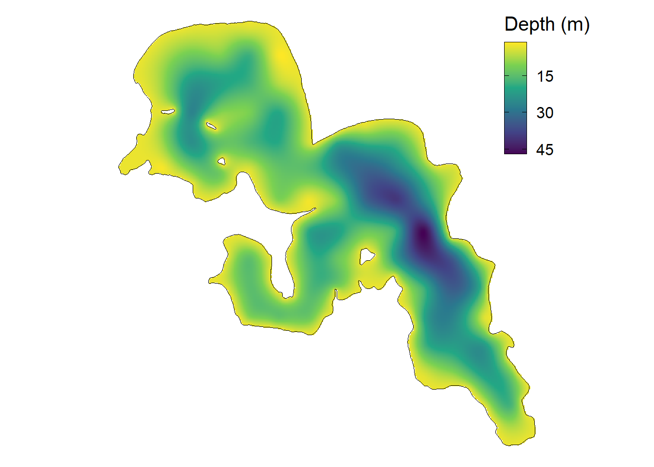
Congratulations! We have made a soap-film GAM that takes in account the boundaries within the lake to estimate the bathymetry of the lake. For this example I used bathymetry, but you can use this workflow to model any type of variable (e.g., fish and/or animal movement/acceleration, wind speed, water quality, ect.)