Estimate trophic position - one source - multiple groups • trps

Our Objectives

The purpose of this vignette is to learn how to estimate trophic position of a species using stable isotope data ( $\delta^{13}C$ and $\delta^{15}N$ ). We can estimate trophic position using a one source model based on equations from Post 2002.

Trophic Position Model

The equation for a one source model consists of the following:

$\text{Trophic Position} = \lambda + \frac{(\delta^{15}N_c - \delta^{15}N_b)}{\Delta N}$

Where $\lambda$ is the trophic position of the baseline (e.g., 2), $\delta^{15}N_c$ is the $\delta^{15}N$ of the consumer, $\delta^{15}N_b$ is the mean $\delta^{15}N$ of the baseline, and $\Delta N$ is the trophic enrichment factor (e.g., 3.4).

To use this model with a Bayesian framework, we need to rearrange this equation to the following:

$\delta^{15}N_c = \delta^{15}N_b + \Delta N \times (\text{Trophic Position} - \lambda)$

The function one_source_model() uses this rearranged equation.

Vignette structure

First we need to organize the data prior to running the model. To do this work we will use {dplyr} and {tidyr} but we could also use {data.table}.

When running the model we will use {trps} and {brms} and iterative processes provided by {purrr}.

Once we have run the model we will use {bayesplot} to assess models and then extract posterior draws using {tidybayes}. Posterior distributions will be plotted using {ggplot2} and {ggdist} with colours provided by {viridis}.

Load packages

First we load all the packages needed to carry out the analysis.

{
library(bayesplot)
library(brms)
library(dplyr)
library(ggplot2)
library(ggdist)
library(grid)
library(purrr)
library(tidybayes)
library(tidyr)
library(trps)
library(viridis)
}

Working with multiple groups

In {trps} we have a data set that has consumer and baseline data already joined for two ecoregions (combined_iso) using the same methods above. Let’s look at this data frame.

Organize data - multiple groups

combined_iso
#> # A tibble: 117 × 13
#>       id common_name ecoregion  d13c  d15n d13c_b1 d15n_b1 d13c_b2 d15n_b2    c1
#>    <int> <fct>       <fct>     <dbl> <dbl>   <dbl>   <dbl>   <dbl>   <dbl> <dbl>
#>  1     1 Lake Trout  Anthropo… -22.3  17.6   -20.3    8.85   -26.4    7.72 -21.3
#>  2     2 Lake Trout  Anthropo… -23.0  17.7   -20.1    8.77   -24.4    8.69 -21.3
#>  3     3 Lake Trout  Anthropo… -21.2  16.7   -20.3    8.85   -24.8    7.99 -21.3
#>  4     4 Lake Trout  Anthropo… -20.9  18.7   -20.1    8.77   -24.4    8.69 -21.3
#>  5     5 Lake Trout  Anthropo… -20.7  18.0   -20.5    8.38   -24.8    7.99 -21.3
#>  6     6 Lake Trout  Anthropo… -20.7  18.0   -20.1    8.34   -24.4    8.05 -21.3
#>  7     7 Lake Trout  Anthropo… -22.8  17.8   -19.7    8.04   -24.1    8.79 -21.3
#>  8     8 Lake Trout  Anthropo… -22.4  17.9   -20.1    8.56   -24.6   10.7  -21.3
#>  9     9 Lake Trout  Anthropo… -20.9  18.4   -18.7    8.95   -24.3   10.6  -21.3
#> 10    10 Lake Trout  Anthropo… -21.7  17.7   -20.8    9.28   -24.6   10.7  -21.3
#> # ℹ 107 more rows
#> # ℹ 3 more variables: n1 <dbl>, c2 <dbl>, n2 <dbl>

We can see that this data frame has isotope data for a second baseline (dreissenids; d13c_b2 and d15n_b2) as well as the mean values for both baselines (c1-n2). These columns for the second baseline are useful when estimating trophic position using a two source model but we do not need them for this analysis and they can be removed.

We can also confirm that this data set has one species, lake trout.

unique(combined_iso$common_name)
#> [1] Lake Trout
#> Levels: Lake Trout

collected from two ecoregions in Lake Ontario.

unique(combined_iso$ecoregion)
#> [1] Anthropogenic Embayment    
#> Levels: Anthropogenic Embayment

Let’s remove the columns we don’t need, d13c_b2, d15n_b2, c2, n2, and add $\lambda$ to the data frame (l1). To do so we make a name column that will be the two groups we have, common_name and ecoregion pasted together. We are doing this to make the iterative processes easier.

combined_iso_update <- combined_iso %>% 
  dplyr::select(-c(d13c_b2, d15n_b2, c2, n2)) %>% 
  mutate(
    l1 = 2, 
    name = paste(ecoregion, common_name, sep = "_")
  ) %>% 
  dplyr::select(id, common_name, ecoregion, name, d13c:l1)

Let’s view our completed data set.

combined_iso_update
#> # A tibble: 117 × 11
#>       id common_name ecoregion     name   d13c  d15n d13c_b1 d15n_b1    c1    n1
#>    <int> <fct>       <fct>         <chr> <dbl> <dbl>   <dbl>   <dbl> <dbl> <dbl>
#>  1     1 Lake Trout  Anthropogenic Anth… -22.3  17.6   -20.3    8.85 -21.3  8.14
#>  2     2 Lake Trout  Anthropogenic Anth… -23.0  17.7   -20.1    8.77 -21.3  8.14
#>  3     3 Lake Trout  Anthropogenic Anth… -21.2  16.7   -20.3    8.85 -21.3  8.14
#>  4     4 Lake Trout  Anthropogenic Anth… -20.9  18.7   -20.1    8.77 -21.3  8.14
#>  5     5 Lake Trout  Anthropogenic Anth… -20.7  18.0   -20.5    8.38 -21.3  8.14
#>  6     6 Lake Trout  Anthropogenic Anth… -20.7  18.0   -20.1    8.34 -21.3  8.14
#>  7     7 Lake Trout  Anthropogenic Anth… -22.8  17.8   -19.7    8.04 -21.3  8.14
#>  8     8 Lake Trout  Anthropogenic Anth… -22.4  17.9   -20.1    8.56 -21.3  8.14
#>  9     9 Lake Trout  Anthropogenic Anth… -20.9  18.4   -18.7    8.95 -21.3  8.14
#> 10    10 Lake Trout  Anthropogenic Anth… -21.7  17.7   -20.8    9.28 -21.3  8.14
#> # ℹ 107 more rows
#> # ℹ 1 more variable: l1 <dbl>

This example data is now ready to be analyzed.

Estimate trophic position - multiple groups

We will use similar structure as before to model trophic position, however, we first split() the data into a list for all groups and then use map() from {purrr} to run the model for each group.

You will notice that the brm() call is exactly the same as when we ran the model for one group. The only difference here is when using map(), the data argument in brm() needs to be replaced with .x to tell brm() where to get the data.

Model - multiple groups

Let’s run the model!

m1 <- combined_iso_update %>% 
  split(.$name) %>% 
  map( ~ brm(
    formula = one_source_model(),
    prior = one_source_priors(),
    stanvars = one_source_priors_params(),
    data = .x,
    family = gaussian(),
    chains = 2,
    iter = 4000,
    warmup = 1000,
    cores = 4,
    seed = 4,
    control = list(adapt_delta = 0.95)
  ), 
  .progress = TRUE
  )
#> Compiling Stan program...
#> Start sampling
#>  ■■■■■■■■■■■■■■■■                  50% |  ETA:  1m
#> Compiling Stan program...
#> Start sampling

Model output - multiple groups

Let’s look at the summary of both models.

m1
#> $`Anthropogenic_Lake Trout`
#>  Family: gaussian 
#>   Links: mu = identity; sigma = identity 
#> Formula: d15n ~ n1 + dn * (tp - l1) 
#>          dn ~ 1
#>          tp ~ 1
#>    Data: .x (Number of observations: 87) 
#>   Draws: 2 chains, each with iter = 4000; warmup = 1000; thin = 1;
#>          total post-warmup draws = 6000
#> 
#> Regression Coefficients:
#>              Estimate Est.Error l-95% CI u-95% CI Rhat Bulk_ESS Tail_ESS
#> dn_Intercept     3.38      0.26     2.88     3.87 1.00     1645     1794
#> tp_Intercept     4.82      0.22     4.44     5.29 1.00     1644     1818
#> 
#> Further Distributional Parameters:
#>       Estimate Est.Error l-95% CI u-95% CI Rhat Bulk_ESS Tail_ESS
#> sigma     0.48      0.04     0.42     0.57 1.00     2124     2125
#> 
#> Draws were sampled using sampling(NUTS). For each parameter, Bulk_ESS
#> and Tail_ESS are effective sample size measures, and Rhat is the potential
#> scale reduction factor on split chains (at convergence, Rhat = 1).
#> 
#> $`Embayment_Lake Trout`
#>  Family: gaussian 
#>   Links: mu = identity; sigma = identity 
#> Formula: d15n ~ n1 + dn * (tp - l1) 
#>          dn ~ 1
#>          tp ~ 1
#>    Data: .x (Number of observations: 30) 
#>   Draws: 2 chains, each with iter = 4000; warmup = 1000; thin = 1;
#>          total post-warmup draws = 6000
#> 
#> Regression Coefficients:
#>              Estimate Est.Error l-95% CI u-95% CI Rhat Bulk_ESS Tail_ESS
#> dn_Intercept     3.37      0.25     2.89     3.86 1.00     1506     1878
#> tp_Intercept     4.54      0.20     4.21     4.96 1.00     1531     1891
#> 
#> Further Distributional Parameters:
#>       Estimate Est.Error l-95% CI u-95% CI Rhat Bulk_ESS Tail_ESS
#> sigma     0.61      0.09     0.47     0.81 1.00     2145     1903
#> 
#> Draws were sampled using sampling(NUTS). For each parameter, Bulk_ESS
#> and Tail_ESS are effective sample size measures, and Rhat is the potential
#> scale reduction factor on split chains (at convergence, Rhat = 1).

We can see that $\hat R$ is 1, meaning that the variance among and within chains are equal (see {rstan} docmentation on $\hat R$ ) and that ESS is quite large for both groups. Overall, this means that both models are converging and fitting accordingly.

Trace plots - multiple groups

Let’s look at the trace plots and distributions. We use iwalk() instead of map(), as iwalk() invisibly returns .x which is handy when you want to call a function (e.g., plot()) for its side effects rather than its returned value. I have also added grid.text() from {grid} to add the group names to each plot.

m1 %>% 
  iwalk(~ {
    plot(.x) 
    grid.text(.y, x = 0.50, y = 0.98)
  })

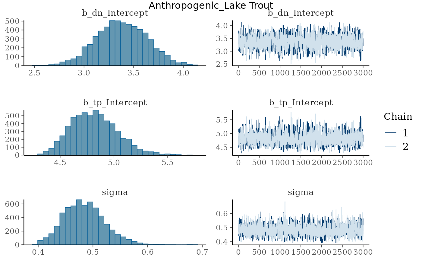
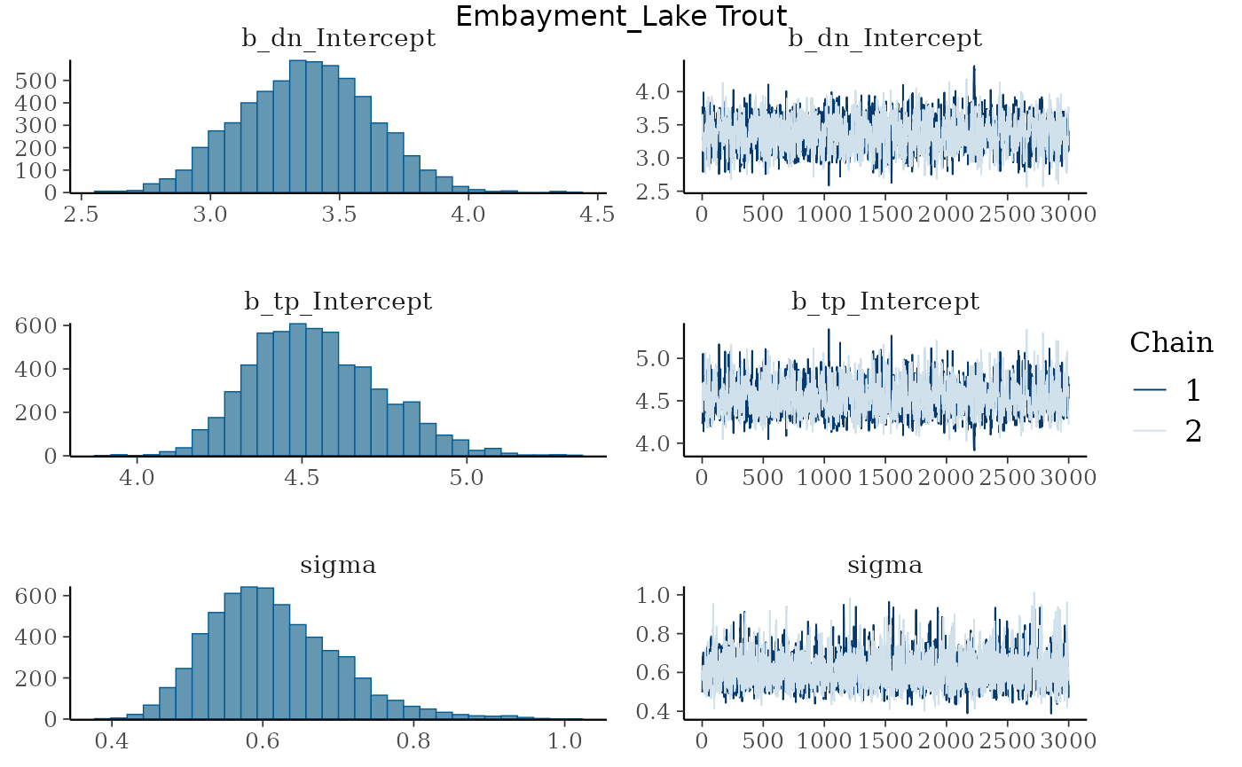
We can see that the trace plots look “grassy” meaning the model is converging!

Posterior draws - multiple groups

Let’s again look at the summary output from the model.

m1
#> $`Anthropogenic_Lake Trout`
#>  Family: gaussian 
#>   Links: mu = identity; sigma = identity 
#> Formula: d15n ~ n1 + dn * (tp - l1) 
#>          dn ~ 1
#>          tp ~ 1
#>    Data: .x (Number of observations: 87) 
#>   Draws: 2 chains, each with iter = 4000; warmup = 1000; thin = 1;
#>          total post-warmup draws = 6000
#> 
#> Regression Coefficients:
#>              Estimate Est.Error l-95% CI u-95% CI Rhat Bulk_ESS Tail_ESS
#> dn_Intercept     3.38      0.26     2.88     3.87 1.00     1645     1794
#> tp_Intercept     4.82      0.22     4.44     5.29 1.00     1644     1818
#> 
#> Further Distributional Parameters:
#>       Estimate Est.Error l-95% CI u-95% CI Rhat Bulk_ESS Tail_ESS
#> sigma     0.48      0.04     0.42     0.57 1.00     2124     2125
#> 
#> Draws were sampled using sampling(NUTS). For each parameter, Bulk_ESS
#> and Tail_ESS are effective sample size measures, and Rhat is the potential
#> scale reduction factor on split chains (at convergence, Rhat = 1).
#> 
#> $`Embayment_Lake Trout`
#>  Family: gaussian 
#>   Links: mu = identity; sigma = identity 
#> Formula: d15n ~ n1 + dn * (tp - l1) 
#>          dn ~ 1
#>          tp ~ 1
#>    Data: .x (Number of observations: 30) 
#>   Draws: 2 chains, each with iter = 4000; warmup = 1000; thin = 1;
#>          total post-warmup draws = 6000
#> 
#> Regression Coefficients:
#>              Estimate Est.Error l-95% CI u-95% CI Rhat Bulk_ESS Tail_ESS
#> dn_Intercept     3.37      0.25     2.89     3.86 1.00     1506     1878
#> tp_Intercept     4.54      0.20     4.21     4.96 1.00     1531     1891
#> 
#> Further Distributional Parameters:
#>       Estimate Est.Error l-95% CI u-95% CI Rhat Bulk_ESS Tail_ESS
#> sigma     0.61      0.09     0.47     0.81 1.00     2145     1903
#> 
#> Draws were sampled using sampling(NUTS). For each parameter, Bulk_ESS
#> and Tail_ESS are effective sample size measures, and Rhat is the potential
#> scale reduction factor on split chains (at convergence, Rhat = 1).

We can see that, for lake trout from the Anthropogenic ecoregion, $\Delta N$ is estimated to be 3.38 with l-95% CI of 2.88, and u-95% CI of 3.87. If we move down to trophic position (tp) we see trophic position is estimated to be 4.82 with l-95% CI of 4.44, and u-95% CI of 5.29.

We can see that, for lake trout from the Embayment ecoregion, $\Delta N$ is estimated to be 3.37 with l-95% CI of 2.89, and u-95% CI of 3.86. If we move down to trophic position (tp) we see trophic position is estimated to be 4.54 with l-95% CI of 4.21, and u-95% CI of 4.96.

Predictive posterior check

We can check how well the model is predicting the $\delta^{15}N$ of the consumer using pp_check() from bayesplot. We have to use map() from purrr to iterate over the list that has our model objects.

m1 %>% 
  map(~ .x %>% 
        pp_check()
  )
#> Using 10 posterior draws for ppc type 'dens_overlay' by default.
#> Using 10 posterior draws for ppc type 'dens_overlay' by default.
#> $`Anthropogenic_Lake Trout`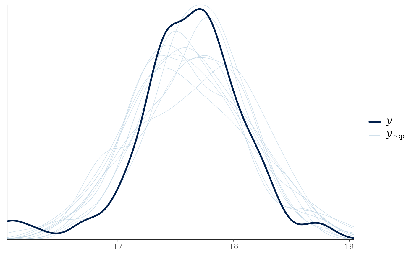

#> 
#> $`Embayment_Lake Trout`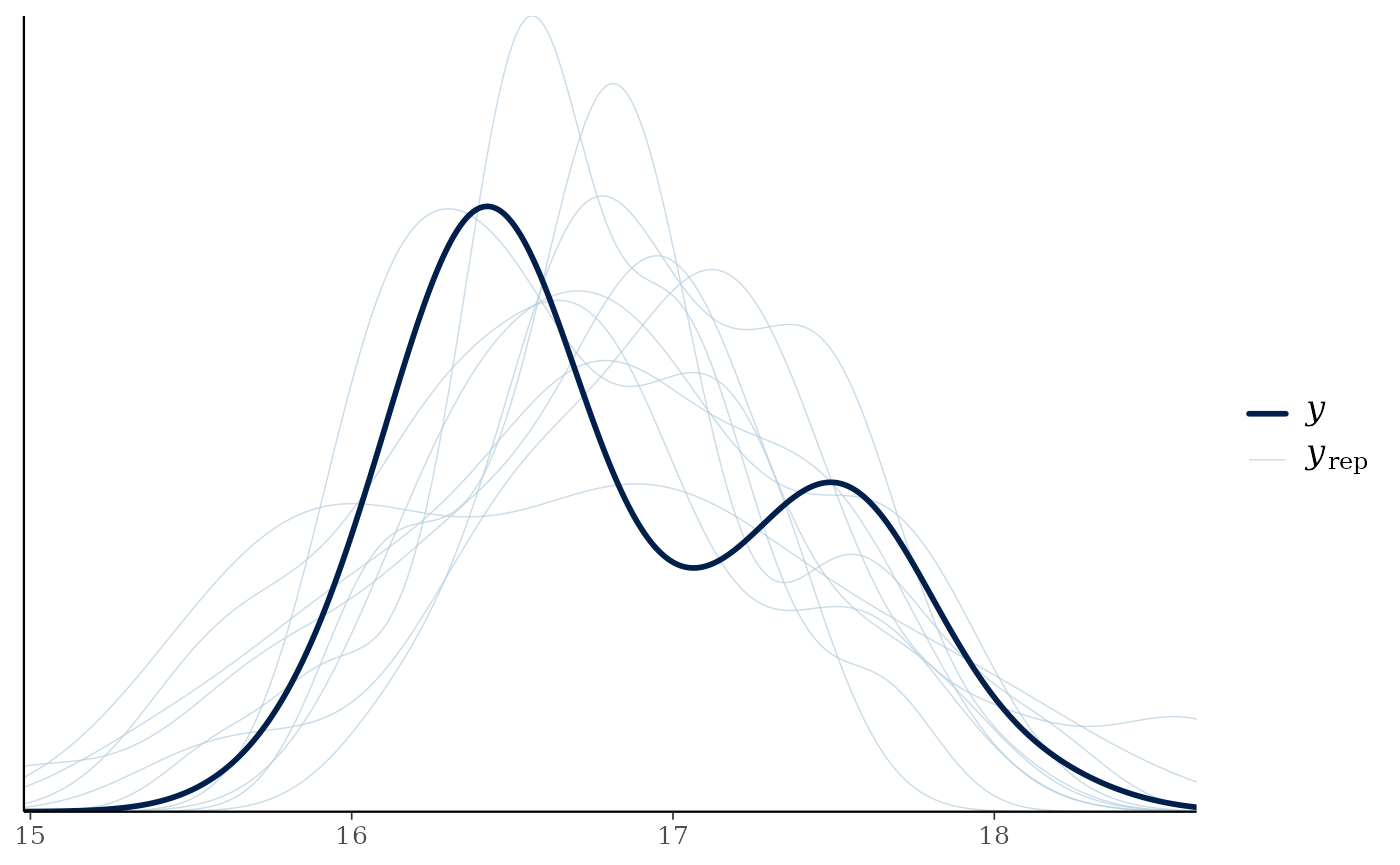

We can see that posteriors draws ( $y_{rep}$ ; light lines) for both groups are are effectively modeling $\delta^{15}N$ of the consumer ( $y$ ; dark line).

Extract posterior draws - multiple groups

We use functions from {tidybayes} to do this work. First we look at the the names of the variables we want to extract using get_variables(). Considering we have multiple models in m1 that all have the same structure, we can just look at the names of the first model object in m1.

get_variables(m1[[1]])
#>  [1] "b_dn_Intercept" "b_tp_Intercept" "sigma"          "lprior"        
#>  [5] "lp__"           "accept_stat__"  "stepsize__"     "treedepth__"   
#>  [9] "n_leapfrog__"   "divergent__"    "energy__"

You will notice that "b_tp_Intercept" is the name of the variable that we are wanting to extract. Next we extract posterior draws using gather_draws(), and rename "b_tp_Intercept" to tp.

Again, considering we have multiple models in m1 we need to use map() to iterate over m1 to get the posterior draws. Once we have iterated over m1 to extract draws we can combine the results using bind_rows() from {dplyr}. The variable name will have the name of the ecoregion and common name of the species pasted to together by a _. We need to separate this string into the two variables we want, being ecoregion and common_name. We can do this by using separate_wider_delim() from {tidyr}. When using this function it will separate the columns and keep them as characters, hence why the last step is to convert ecoregion into a factor.

For your data you will likely have category names other than ecoregion and common_name. Please replace with the columns that fit your data structure.

post_draws_mg <- m1 %>%
  map(~ .x %>% 
        gather_draws(b_tp_Intercept) %>% 
        mutate(
          .variable = "tp"
        ) %>% 
        ungroup()
  ) %>% 
  bind_rows(.id = "name") %>% 
  separate_wider_delim(name, names = c("ecoregion", "common_name"), 
                       delim = "_", cols_remove = FALSE) %>% 
  mutate(
    ecoregion = factor(ecoregion, 
                       levels = c("Anthropogenic", "Embayment")), 
  )

Let’s view the post_draws_mg

post_draws_mg
#> # A tibble: 12,000 × 8
#>    ecoregion     common_name name       .chain .iteration .draw .variable .value
#>    <fct>         <chr>       <chr>       <int>      <int> <int> <chr>      <dbl>
#>  1 Anthropogenic Lake Trout  Anthropog…      1          1     1 tp          4.49
#>  2 Anthropogenic Lake Trout  Anthropog…      1          2     2 tp          4.90
#>  3 Anthropogenic Lake Trout  Anthropog…      1          3     3 tp          4.74
#>  4 Anthropogenic Lake Trout  Anthropog…      1          4     4 tp          4.87
#>  5 Anthropogenic Lake Trout  Anthropog…      1          5     5 tp          4.86
#>  6 Anthropogenic Lake Trout  Anthropog…      1          6     6 tp          5.17
#>  7 Anthropogenic Lake Trout  Anthropog…      1          7     7 tp          5.16
#>  8 Anthropogenic Lake Trout  Anthropog…      1          8     8 tp          5.11
#>  9 Anthropogenic Lake Trout  Anthropog…      1          9     9 tp          4.94
#> 10 Anthropogenic Lake Trout  Anthropog…      1         10    10 tp          4.95
#> # ℹ 11,990 more rows

We can see that the posterior draws data frame consists of seven variables:

ecoregion
common_name
.chain
.iteration (number of samples after burn-in)
.draw (number of samples from iter)
.variable (this will have different variables depending on what is supplied to gather_draws())
.value (estimated value)

Note - the names of and items in the first two columns will vary depending on the names you split your data into.

Extracting credible intervals - multiple groups

Considering we are likely using this information for a paper or presentation, it is nice to be able to report the median and credible intervals (e.g., equal-tailed intervals; ETI). We can extract and export these values using spread_draws() and median_qi from {tidybayes}.

Again, because m1 is a list of our model objects, we need to map() over the list to calculate these values. Then we do the same procedures we have done before to combine and restructure the outputs. Lastly, we use mutate_if() to round all columns that are numeric to two decimal points.

post_medians_ci <- m1 %>%
  map(~ .x %>% 
        spread_draws(b_tp_Intercept) %>%
        median_qi() %>% 
        rename(
          tp = b_tp_Intercept
        ) 
  ) %>% 
  bind_rows(.id = "name") %>% 
  separate_wider_delim(name, names = c("ecoregion", "common_name"), 
                       delim = "_", cols_remove = FALSE) %>% 
  mutate(
    ecoregion = factor(ecoregion, 
                       levels = c("Anthropogenic", "Embayment")), 
  ) %>% 
  mutate_if(is.numeric, round, digits = 2)

Let’s view the output.

post_medians_ci
#> # A tibble: 2 × 9
#>   ecoregion     common_name name        tp .lower .upper .width .point .interval
#>   <fct>         <chr>       <chr>    <dbl>  <dbl>  <dbl>  <dbl> <chr>  <chr>    
#> 1 Anthropogenic Lake Trout  Anthrop…  4.81   4.44   5.29   0.95 median qi       
#> 2 Embayment     Lake Trout  Embayme…  4.53   4.21   4.96   0.95 median qi

I like to use {openxlsx} to export these values into a table that I can use for presentations and papers. For the vignette I am not going to demonstrate how to do this but please check out openxlsx.

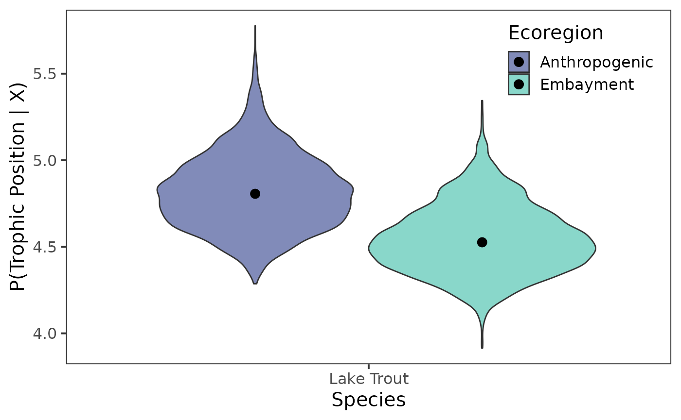
Plotting posterior distributions - multiple groups

Now that we have our posterior draws extracted we can plot them. For comparing trophic position among species or groups, I like using either violin plots, interval points, or slab plots for posteriors. We can access violins through {ggplot2} with the later being available in {ggdist}.

Violin plot

Let’s first look at the violin plot.

ggplot(data = post_draws_mg, aes(x = common_name, 
                                 y = .value, 
                                 fill = ecoregion)) + 
  geom_violin() + 
  stat_summary(fun = median, geom = "point", 
               size = 3, 
               position = position_dodge(0.9)
  ) + 
  scale_fill_viridis_d(name = "Ecoregion", 
                       option = "G", 
                       begin = 0.35, 
                       end = 0.75, alpha = 0.65) + 
  theme_bw(base_size = 15) + 
  theme(
    panel.grid = element_blank(),
    legend.position = "inside", 
    legend.position.inside = c(0.85, 0.86)
  ) +
  labs(
    x = "Species", 
    y = "P(Trophic Position | X)"
  )

Point interval plot

Next, we’ll look at the point interval plot – but first we need to create our colour palette.

viridis_colours <- viridis(2,
                           option = "G",
                           begin = 0.35, 
                           end = 0.75, 
                           alpha = 0.65)

Now let’s plot the point intervals.

ggplot(data = post_draws_mg, aes(x = common_name, 
                                 y = .value, 
                                 group = ecoregion)) + 
  stat_pointinterval(
    aes(point_fill = ecoregion),
    point_size = 4,
    interval_colour = "grey60",
    position = position_dodge(0.4),
    shape = 21,
  ) + 
  scale_fill_manual(aesthetics = "point_fill",
                    values = viridis_colours,
                    name = "Ecoregion") +
  theme_bw(base_size = 15) + 
  theme(
    panel.grid = element_blank(),
    legend.position = "inside", 
    legend.position.inside = c(0.85, 0.86)
  ) +
  labs(
    x = "Species", 
    y = "P(Trophic Position | X)"
  )

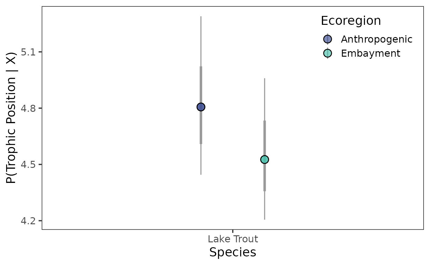
Congratulations we have successfully run a Bayesian one source trophic position model for one species in two ecoregions of Lake Ontario!